The often-overlooked random forest kernel
Machine learning problems often require a kernel function that measures the similarity between two different input vectors, and . Such kernel functions can enable linear algorithms (like SVM, PCA, and k-means) to find non-linear solutions to classification, regression, or clustering problems. Normally, a kernel function is selected from a standard set (although the most common by far appears to be the radial basis function) and tuned slightly based on the dataset. Here, we’ll discuss a type of kernel called the random forest kernel, which takes advantage of a pre-trained random forest in order to provide a custom-tailored kernel.
The Colonel’s Cocktail Party
Imagine you are a decorated colonel who hosts an annual cocktail party. Your guests mingle and periodically shift between groups of their peers, all the while admiring your tasteful mid-century decoration and savoring delicious hor d’oeuvres.
You, being both a subtle and naturally curious colonel, wish to determine whether or not two of your guests (guest 3 and guest 6) have any “affinity” for each other. However, to avoid detection, you cannot intervene. Observe the cocktail party below.
| Portion 3 and 6 are together: | 0.00 |
| Portion 1 and 4 are together: | 0.00 |
| Average togetherness: | 0.00 |
You keep track of how often guest 3 and guest 6 appear in the same group and compare that against how often two other guests (1 and 4), and the average guest, appear in the same group. As the party progresses, what can you, the colonel, conclude about the affinity guests 3 and 6 have for being in the same group?
We can think of each timestep of the cocktail party as a random partition of your guests. At any particular time , the five sets of party-goers are disjoint (assume invitees move between tables instantly). If there is an affinity for one individual to end up in the same group as another individual , then the percentage of time that we see and together will be higher than the average number of times we see every distinct pair together. If we define:
… then can be used a measure of affinity for and . The higher the value of , the higher the affinity between and . It turns out that can be used as a kernel function: specifically, given a set of partitionings, the function will produce a positive semidefinite Gram matrix. The specific mathematical requirements are interesting, but it suffices to accept that this is a sufficient and necessary condition for to be used as a kernel function.
The question then becomes: how does one create a set of partionings such that elements that are similar (in some context) are frequently grouped together? One can find answers in both Geurts et al. and Davies et al., but the short answer is to use a random forest!
Random Forest Kernel
Random forests are a powerful machine learning ensemble method that combine the results of several decision (or regression) trees into a single model. Consider the example below.
The two-forest random forest shown above has been trained on some dataset, and we can now use it to classify new vectors. Consider the vectors , , , and . You can touch or hover over a vector to see how the forest classifies it.
To use the random forest as a kernel, we view each level of each tree as a partitioning. For example, the first level of the first tree (left hand side) partitions potential vectors into two groups, and . The second level of second tree (right hand side) partitions potential vectors into four groups, , , , and . The random forest kernel, , is the number of times and fall into the same partition divided by the total number of partitionings.
The above tree contains five different partitionings. We can thus evaluate by counting the number of times they share a partition. Since and share all but one partition, . Since and share no partitions in common, the kernel is zero, i.e. .
If two items are in the same partition frequently, they are guaranteed to share some properties (i.e. their values share a set of constraints), but because the random forest is built using semantic information (e.g., the class or label of the data), these groupings of properties will have semantic meaning. Thus, items that share more partitions are more similar, and items that share few partitions are dissimilar.
Examples
It might seem odd to train a random forest model on a dataset and then use that random forset as a kernel, instead of using the random forest directly. However, this can be useful in a number of circumstances.
For example, consider the MNSIT digit recognition dataset. A large random forest can obtain acceptable (greater than 90% accuracy) if it is trained on all ten digit classes. In other words, if the random forest algorithm is allowed to see many examples of each digit class, it can learn to classify each of the ten digits. But what if the random forest algorithm is only allowed to see examples of 7s and 9s? Clearly, such a random forest would not be very useful on a dataset of 3s and 4s. However, using the random forest kernel, we can take advantage of a random forest trained on only 7s and 9s to help us understand the differences between 3s and 4s (this is often called transfer learning).
Consider two different PCA projections of the 3s and 4s from the MNIST dataset:
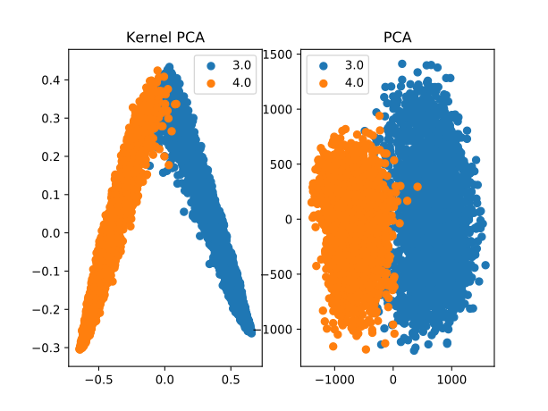
The left-hand side image shows the results of using Kernel PCA to find the two most significant (potentially non-linear) components of the 3s and 4s data using the random forest kernel. The right-hand side shows the two most significant (linear) components as determined by PCA.
For the most part, the components found using the random forest kernel provide a much better separation of the data. Remember, the random forest here only got to see 7s and 9s – it has never seen a 3 or a 4, yet the partitions learned by the random forest still carry semantic meaning about digits that can be transferred to 3s and 4s.
In fact, if one trains an SVM model to find a linear boundary on the first 5 principal components of the data, the accuracy for the random forest kernel assisted PCA + SVM is 94%, compared to the 87% of the linear PCA + SVM scheme.
The random forest kernel can be a quick and easy way to transfer knowledge from a random forest model to a related domain when techniques like deep belief nets are too expensive or simply overkill. The kernel can be evaluated quickly, and does not require special hardware or a significant amount of memory to compute. It isn’t frequently useful, but it is a nice trick to keep in your back pocket.
Notes
The metaphor of the cocktail party in this context was first introduced by A. Davies and Z. Ghahramani in their paper, “The Random Forest Kernel and other kernels for big data from random partitions” (available on arXiv). They explain:
We consider The Colonel, who is the host of a cocktail party. He needs to determine the strength of the affinity between two of his guests, Alice and Bob. Neither Alice and Bob, nor the other guests, must suspect the Colonel’s intentions, so he is only able to do so through surreptuous (sic) observation.
At the beginning of the evening, his N guests naturally form into different groups to have conversations. As the evening progresses, these groups naturally evolve as people leave and join different conversations. At m opportunities during the course of the evening, our host notes whether Alice and Bob are together in the same conversation.
As the Colonel farewells his guests (sic), he has a very good idea of Alice and Bob’s affinity for one another.