Pretty pictures with perlin noise fields

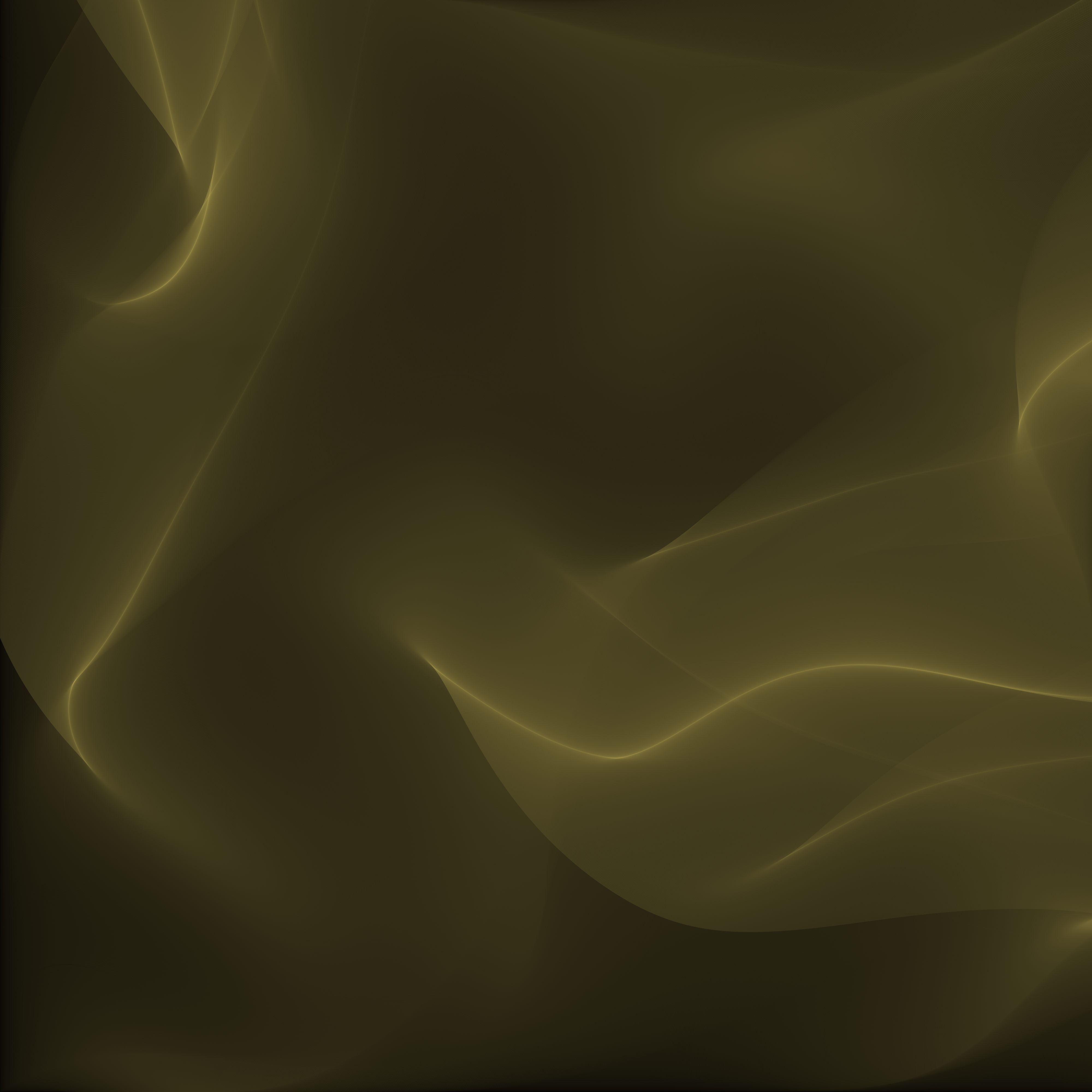
Perlin noise can be used to create some interesting and fun visual effects, like the image below (click for high resolution):

The above image was created by interpreting each point in 2D Perlin noise as an angle in a vector field, and then tracing particles through the resulting vector field. Each pixel is colored based on its flux. In order to explain how it is built, we’ll go over the basics of Perlin noise, and flow field particle tracing. You can check out the code on GitHub.

Perlin noise

Perlin noise was invented by Ken Perlin in 1983, and it didn’t take long before it became widely used in computer graphics applications.

Part of what makes Perlin noise so appealing is that it is:

• random, meaning that it exhibits a lot of diversity,
• smooth, meaning that there are no sharp edges or unnatural bumps,
• and globally structured, meaning that it appears to have features and properties that span the whole image.

The first step of generating 2D Perlin noise is creating a lattice of grid points, and randomly assigning one of eight possible vectors to each point. These possible vectors correspond to the cardinal and ordinal directions: north, northeast, east, southeast, south, southwest, west, northwest. For example, a 3x3 grid might look like this:

After generating the grid, Perlin noise is generated in a point-wise fashion. For a given point , we draw vectors , , , and from the point to the nearest four grid points (see the demonstration below). We call the random vectors assigned to the nearest four grid points , , , and . We then compute four dot products – , , , and – between the randomly drawn vectors at each grid point and the distance vectors from our point to each grid point. For example, we have: .

Once we’ve computed , , , and , we use linear interpolation, commonly referred to in computer graphics applications as , in order to combine the dot product values. Linear interpolation is defined as:

The values and are interpolated between, and the value is a weight – higher values of bias the interpolation towards , whereas lower values of bias the intrpolation towards . The basic strategy for picking the color of a point was to compute the dot products, and then interpolate between the dot product of the top two sets of vectors, and , weighted based on the horizontal distance of the point to be colored to the grid points. This weighted value is called . The value is computed similarly for the bottom two sets of vectors (i.e., by interpolating between and ). Finally, the value of a pixel, , is computed by interpolating between and , this time weighting the interpolation by the vertical distance from the point to be colored to the grid points.

However, Perlin found this simple form of interpolation didn’t quite work well enough – it produced overly smooth images. As a result, Perlin first “fades” the weight values for each interpolation with the following function:

The demonstration below shows all the quantities described above for the point depicted. You can use your mouse to select a specific point as well.

Since the vectors at each grid point are selected randomly, the dot product values have diverse properties. Notice how the color value only changes a little bit between two neighboring points – this gives Perlin noise a “smooth” look. By changing the size of the grid, one can control the size of features (i.e., global structures) of the noise.

The four images below show Perlin noise with a grid size of (starting from the top left) 3, 4, 5, and 6.

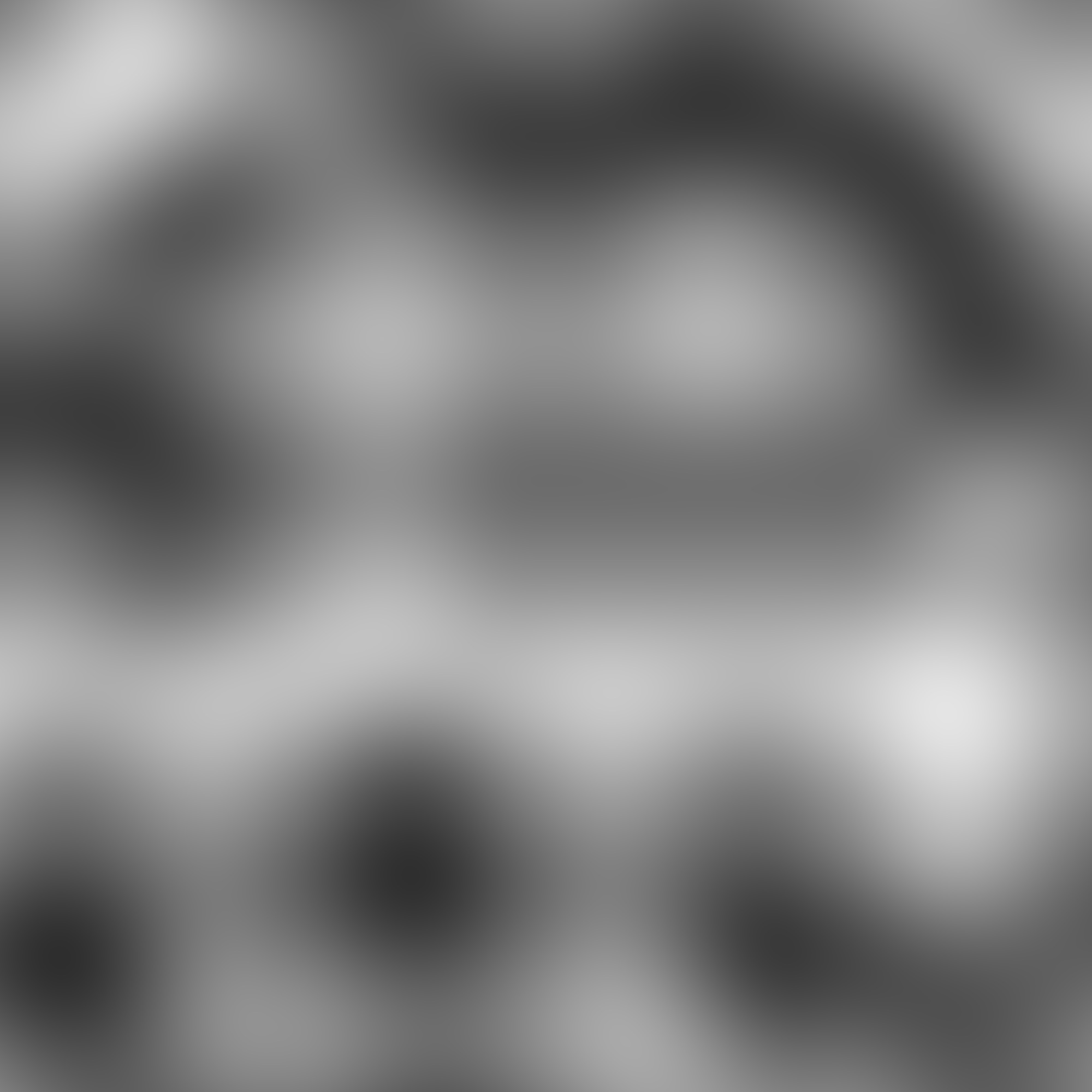
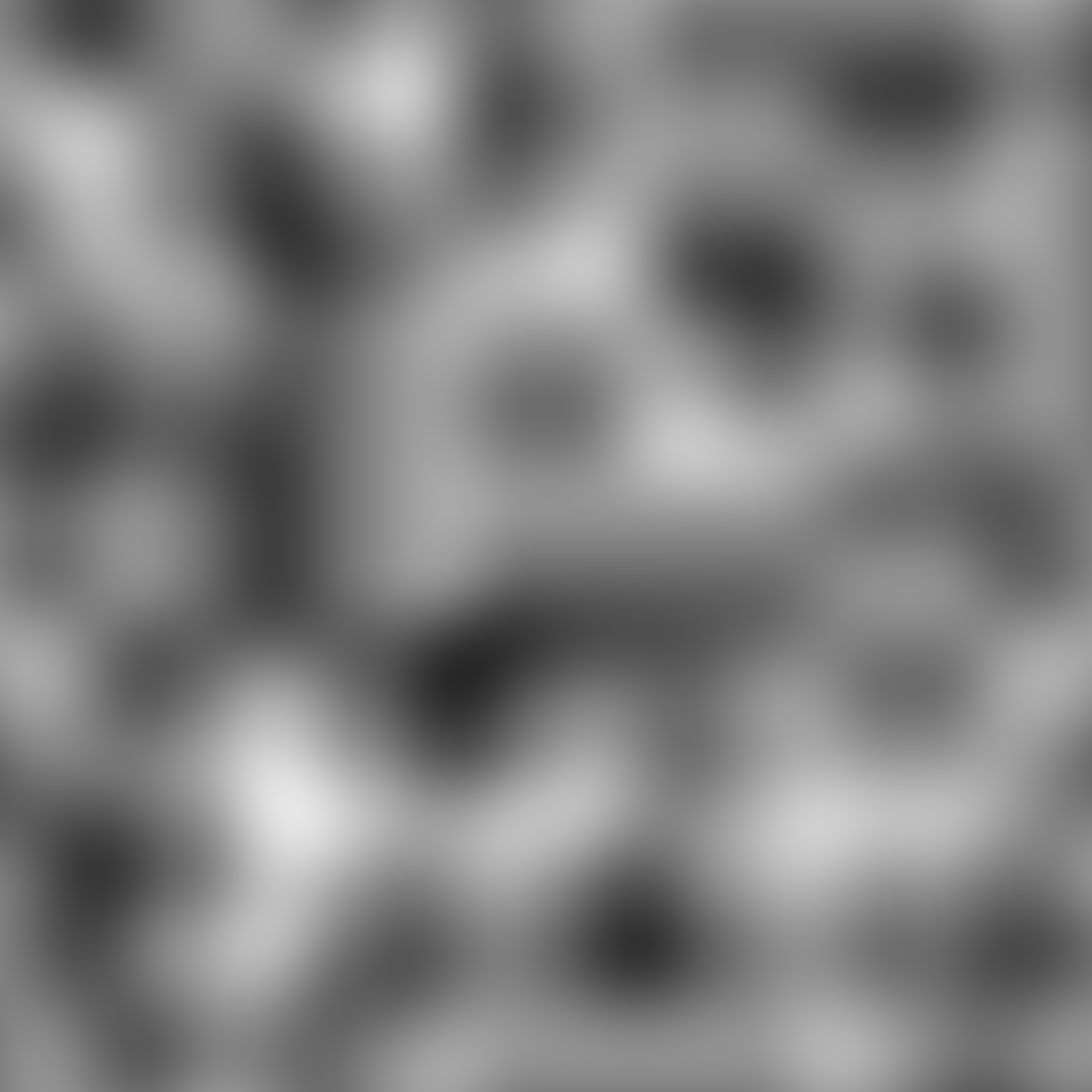
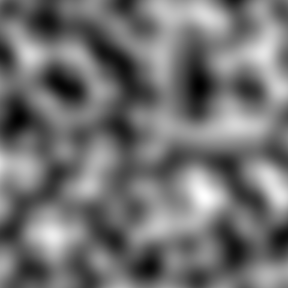
The grid size of Perlin noise is oftern referred to as the frequency of the noise, since higher values correspond to more details and finer-grained edges (and thus the higher frequency components of the image). Multiple frequencies can be combined together into a single image (normally, frequencies that are a power of two, or octaves, are chosen) in order to create multi-level structures:

You can also extend Perlin noise into three dimensions by creating a grid of cubes instead of a grid of squares. You’ll have 6 vectors instead of 4, but the procedure is essentially the same. You could extend Perlin noise to even higher dimensions, although the results might be difficult to interpret.

While Perlin noise values are normally converted directly into pixel values, as we’ve seen so far, we’ll next look at using each Perlin noise value as an angle in a vector field.

Vector fields

A vector field is a simple concept – essentially, a function mapping a point in space to a vector. These vectors can represent a lot of different things, but a very popular use of vector fields is representing velocities. The image below shows a vector field with particles tracing through it.

The plot next to the vector field shows the normalized flux of the vector field – the brightest pixel represents the cell that has seen the largest number of particles travel through it. The plot reset every twenty seconds, but you can also click here to reset it manually.

The implementation is pretty straightforward – an array holds the coordinates of each particle, and at every timestep the position of each particle is incremented by the vector indicated by the vector field. When particles go out of bounds, they are removed.

Turns out, we can interpret Perlin noise itself as a flow field! By considering the value of each point to be an angle instead of a color, converting between the two is trivial. Doing this, plotting the normalized flux, and then choosing a few fun coloring functions can yield some pretty pictures:

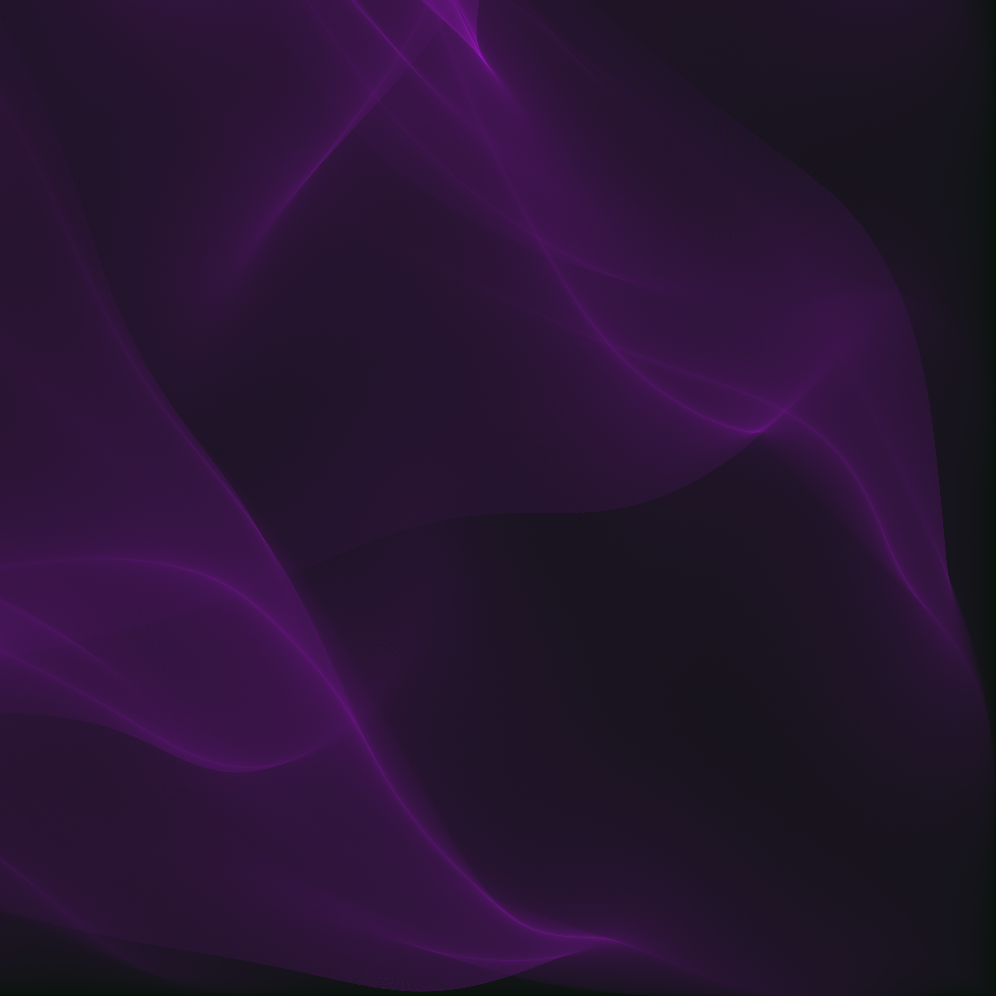
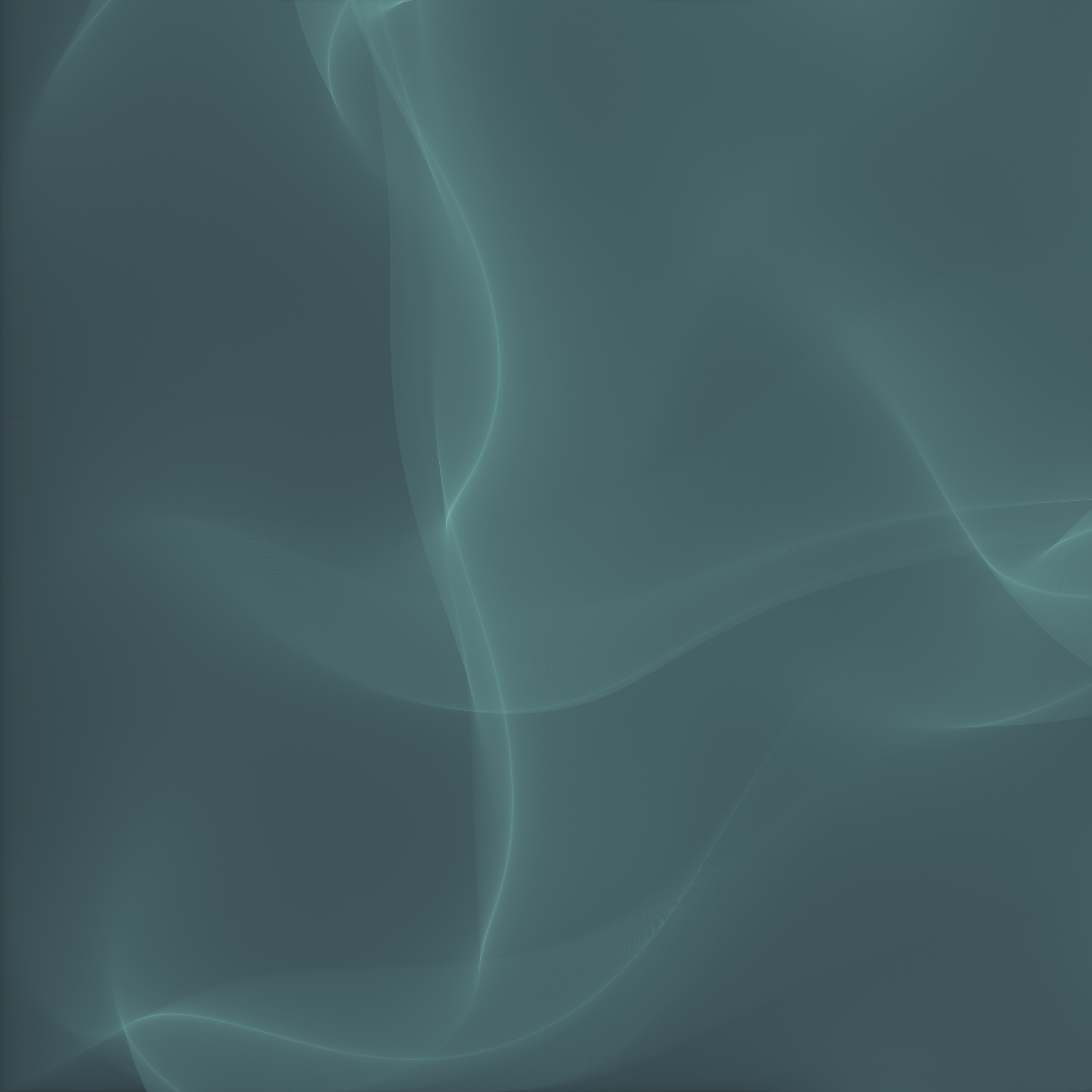
We can also make a video of the flux plot as it builds over time, which can look a bit like a fluid permeating through space.

You can see the full quality video here.

Full quality

Full quality

Full quality

All of the examples in this blog post can be generated with my Perlin noise Rust implementation, which is open source. Check out the repository for exact details on the algorithm.

Other types of noise

Noise is generally defined as an unknown and random modification to a signal. For example, static in the background of an audio recording or TV “snow” may be considered noise. One of the simplest types of noise, white noise, is just values drawn uniformally (often, from the range ). We can plot white noise as an image:

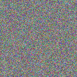
Here, each channel of each pixel is just a random value. The following Python program will generate it:

import numpy as np
import skimage.io
img = np.random.rand(256, 256, 3)
skimage.io.imsave("noise.png", img)

White noise is simple enough, but it isn’t useful because it doesn’t really look like anything. Researchers in computer graphics have been studying how to procedurally (i.e., with a computer) generate “natural” looking noise. One such attempt is Perlin noise, as we’ve seen, but there’s also Worley noise, which can often look like stone, water, or cells. With a little work, we can make it look like it is 3D:

For more examples of Worley noise, click here.

Notes

1. The best explaination of how to generate Perlin noise I’ve seen so far comes from Adrian Biagioli, who’s got a ton of cool projects.
2. You can read the original Perlin noise paper, “An Image Synthesizer”, and the second paper improving on the original algorithm.
3. I first saw the use of Perlin noise as a vector field on Andy Saia’s blog. You can find him on Twitter.